
Classic ecological models in Stan: two-species Levins metapopulation model (mutualism version)
In this post, I cover how to fit a version of the two-species Levins metapopulation model in Stan, as well as how to use R to simulate data to fit the model to.
Acknowledgements and other resources
I relied on several resources when writing this post.
The first is Levins’ classic paper which introduced the single species metapopulation model. I also found this paper by Rampal Etienne to be very useful. The main resource that I used for the two-species metapopulation model was Theoretical Ecology: Principles and Applications, edited by Robert May and Angela McLean - chapter 4, metapopulations and their spatial dynamics by Sean Nee, is the relevant chapter.
I learned about Stan and Bayesian stats in general from Richard McElreath’s book and course Statistical Rethinking, Michael Betancourt’s introduction to Stan, the Stan manual, this post about (relatively) recent changes to the ODE interface and this tutorial by Mikhail Popov.
I also learned a lot about modeling from the book a biologist’s guide to mathematical modeling in ecology and evolution by Sarah Otto and Troy Day.
Disclaimer
I’m mainly writing this post because a) it’s fun and b) it helps me to learn more about the material - if people find it helpful, then that’s even better!
Please bear in mind that there might be mistakes lurking in this post - if you spot any, I’d appreciate if you let me know via email (my address is in the sidebar) or in the comments below. As usual, use of the model etc. is at your own risk.
Introducing the models
Levins’ single-species metapopulation model
Imagine a landscape where there are patches of habitat, each occupied by a population of a species. As some of these populations go extinct patches become empty, and empty patches are colonised by new populations which establish when individuals disperse in from occupied patches. We can study how the population of these populations - the metapopulation - rises and falls over time.
In Levins’ classic paper, he describes the changing metapopulation using the following equation:
\[\frac{dN}{dt} = MN\left(1 - \frac{N}{T} \right) - EN\]where $N$ is the number of occupied patches, $M$ is the migration (or colonisation) rate, $E$ is the extinction rate, and $T$ is the total number of occupiable patches in the landscape.
Looking at the model, it seems oddly familiar… If we sub in a new parameter $r$ which represents the difference between the migration and extinction rates, i.e. $r = M - E$, we see why:
\[\frac{dN}{dt} = rN\left(1 - \frac{N}{T} \right)\]This is just the logistic population growth model that we looked at in the last post! The only difference is that what used to be called the carrying capacity $K$ is now called the total number of occupiable patches $T$.
Since we’ve already looked at this model, we’re going to move on to look at one of the ways that the classic metapopulation model can be extended to two species.
Two-species metapopulation model - mutualism version
There are a variety of ways that the single-species metapopulation model can be extended to two species - several different extensions are described by Sean Nee in chapter 4 of Theoretical Ecology: Principles and Applications. In one version, the two species are mutualists: one species (the “plant”) can exist alone on a patch, but must be dispersed to new patches by the other species (the “disperser”). The disperser cannot survive on a patch by itself, and can only inhabit patches which are occupied by the plant.
Here is the two-species mutualism model as described in ch. 4 of Theoretical Ecology:
\[\frac{dx}{dt} = e_{p}y + e_{d}z - c_{p}zx\\ \frac{dy}{dt} = c_{p}zx - c_{d}zy - e_{p}y\\ \frac{dz}{dt} = c_{d}zy - e{d}z\]Although it’s a two species model, we’re actually tracking the changes in three variables - the proportion of empty sites ($x$), sites with only the plant ($y$), and sites with both the plant and disperser ($z$). We also have two colonisation rate parameters ($c_p$ and $c_d$) and two extinction rate parameters ($e_p$ and $e_d$) which control the shifts between the system’s states.
I am a fan of Otto & Day’s technique of representing ODE’s as flow diagrams, where each variable is represented as a node (circle) and the flows between them are represented as arrows. This is the flow diagram corresponding to the equations above:
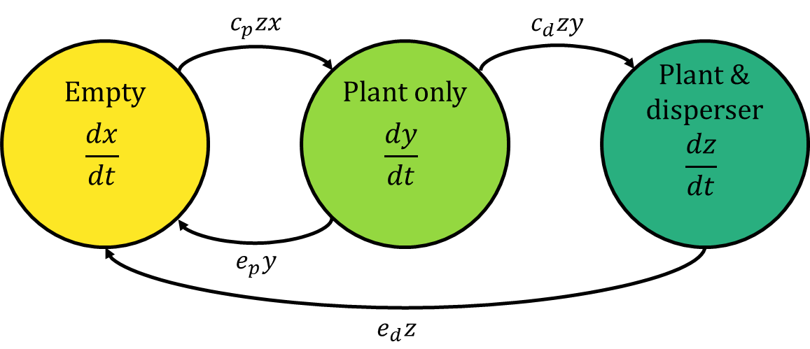
I find that this diagram makes some of the model’s assumptions much clearer. First, there is no arrow going directly from the “empty” node to the “plant & disperser” node. This means that empty patches have to be colonised by the plant before the disperser is able to colonise too - a patch can’t go from empty to containing both species in a single leap.
Second, the flow of patches from empty to the plant-only state is $c_{p}zx$. Notice that $y$ isn’t involved, meaning that if there are no patches with both the plant and disperser, then no new patches can be colonised by the plant - without the disperser, the plant will go extinct!
Finally, there isn’t an arrow from the “plant & disperser” node back to the “plant only” node - this means that once patches contain both species, they never lose only the disperser and return to a plant-only state. Thus, $e_{d}$ really represents the extinction rate of patches with the plant-disperser pair.
Simulating the two-species model in R
Let’s start by loading a couple of packages and setting the seed for the random number generator:
library(rethinking)
library(deSolve)
library(plotly) # only needed for 3d phase diagram plot
set.seed(946)
Now we’re going to write the function which contains our differential equations:
twosp_mutual <- function(times,y,parms){
  X <- y[1]
  Y <- y[2]
  Z <- y[3]

  with(as.list(p),{
    dx.dt <- ep*Y + ed*Z - cp*Z*X
    dy.dt <- cp*Z*X - cd*Z*Y - ep*Y
    dz.dt <- cd*Z*Y - ed*Z

    return(list(c(dx.dt, dy.dt, dz.dt)))
  })
}
After this, we have to pick values for our extinction and colonisation rate parameters - there’s no particular reason for choosing the ones that I did, and you can play around with other values if you like. We also have to pick values for our initial conditions - I went for 90% empty patches, no patches with plants only, and 10% patches with both species. Finally, we have to pick a time sequence for our simulation:
# Extinction and colonisation parameters
ep <- 1 # Plant extinction rate
ed <- 0.5 # Disperser extinction rate
cp <- 4 # Plant colonisation rate
cd <- 5 # Disperser colonisation rate

p <- c(ep=ep, ed=ed, cp=cp, cd=cd) # Make a vector of all of the parameters

# Initial conditions - most patches empty, small proportion have both species
y0 <- c(X = 0.9,
        Y = 0,
        Z = 0.1)

# Time sequence
time <- seq(0,10,by=0.1)
Now we’ve chosen our values, we can use the ode function in the deSolve package to get our metapopulation’s true state at each time step:
state_true <- ode(y=y0, times=time, func = twosp_mutual, parms = p)
We can now visualise how the proportion of patches which are in each state changes over time:
par(mfrow=c(1,3))
plot(X ~ time, data=state_true, type="l", ylim=c(0,1), ylab="Proportion of patches", main="Empty")
plot(Y ~ time, data=state_true, type="l", ylim=c(0,1), ylab="Proportion of patches", main="Plant only")
plot(Z ~ time, data=state_true, type="l", ylim=c(0,1), ylab="Proportion of patches", main="Plant & Disperser")
par(mfrow=c(1,1))
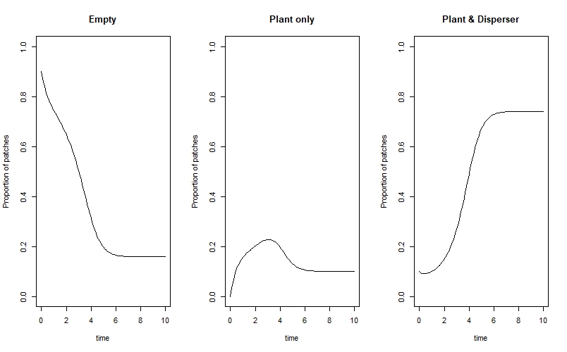
We can see that the system eventually reaches an equilibrium where the majority of patches are occupied by both the plant and disperser, and a smaller proportion are either empty or contain only the plant.
Just for fun, we can plot the state of the whole system over time as a 3D phase-space diagram - this code will produce an interactive plot which you can click and drag to rotate in the plot viewer:
fig <- plot_ly(as.data.frame(state_true), x = ~X, y= ~Y, z= ~Z, type = "scatter3d", mode="lines",
               line = list(width = 6, color = ~time, reverscale = FALSE, colorscale = "Viridis"))
fig
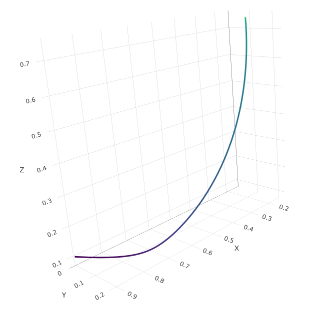
We can see the system track a path from the initial conditions in the bottom left, to the final equilibrium in the top right.
Now that we’ve simulated the system’s true underlying state, we can simulate the observation processes which will produce the actual data that we’re going to fit the model to. Since my main focus here was on learning about coding a model with more than one ODE, I went for a relatively simple observation process. The idea is we observe a finite number of sites (I went for 1000) and the number of sites in each state at a given time follows a multinomial distribution where the probabilities of each state are the true proportions contained in state_true. The code goes like this:
  n_sites <- 1000 # Number of sites observed

  counts_obs <- matrix(NA, nrow = length(time), ncol = 3)
  for(i in 1:length(time)){
    counts_obs[i,] <- rmultinom(n = 1, size = n_sites, prob = state_true[i, 2:4])
  }
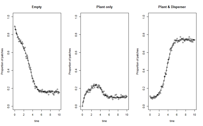
The result is a matrix, counts_obs, which holds the number of sites in each state (empty, plant only, plant & disperser) at each time step.
We can plot the observed data on top of our true state lines from above like this:
par(mfrow=c(1,3))
plot(X ~ time, data=state_true, type="l", ylim=c(0,1), ylab="Proportion of patches", main="Empty")
points(x = time, y=counts_obs[,1]/n_sites)
plot(Y ~ time, data=state_true, type="l", ylim=c(0,1), ylab="Proportion of patches", main="Plant only")
points(x = time, y=counts_obs[,2]/n_sites)
plot(Z ~ time, data=state_true, type="l", ylim=c(0,1), ylab="Proportion of patches", main="Plant & Disperser")
points(x = time, y=counts_obs[,3]/n_sites)
par(mfrow=c(1,1))
Finally, we can prepare our data list for Stan. Just like in the post on exponential and logistic population growth, we have to separate the initial time step from the rest of the time series - this is because of the way that Stan indexes time steps. The code is:
dlist <- list(
  n_times = length(time)-1L,
  y0_obs = counts_obs[1,],
  y = counts_obs[-1,],
  t0 = 0,
  ts = time[-1],
  n_sites = as.integer(n_sites)
)
Coding the model in Stan
Now that we’ve simulated the data, we can code the Stan model!
Here is the full model:
functions{
  vector exp_growth(real t, // Time
                    vector y, // State
                    real ep, // Plant extinction rate
                    real ed, // Disperser extinction rate
                    real cp, // Plant colonisation rate
                    real cd){ // Disperser colonisation rate
    vector[3] dndt;
    dndt[1] = ep*y[2] + ed*y[3] - cp*y[3]*y[1]; // Empty patches
    dndt[2] = cp*y[3]*y[1] - cd*y[3]*y[2] - ep*y[2]; // Plant-only patches
    dndt[3] = cd*y[3]*y[2] - ed*y[3]; // Both species patches
    return dndt;
  }
}
data {
  int<lower=1> n_times; // Number of time steps minus one
  array[n_times, 3] int<lower=0> y; // Observed data, minus initial state
  array[3] int<lower=0> y0_obs; // Observed initial state
  real t0; // First time step
  array[n_times] real ts; // Time steps
  int<lower=0> n_sites; // Number of sites
}
parameters {
  simplex[3] y0; // Initial state (must sum to 1)
  real<lower=0> ep; // Plant extinction rate
  real<lower=0> ed; // Disperser extinction rate
  real<lower=0> cp; // Plant colonisation rate
  real<lower=0> cd; // Disperser colonisation rate
}
transformed parameters{
    // ODE solver
  simplex[3] theta[n_times] = ode_rk45(exp_growth, y0, t0, ts, ep, ed, cp, cd);
}
model {
  // Priors
  ep ~ exponential(0.5); // Plant extinction rate
  ed ~ exponential(0.5); // Disperser extinction rate
  cp ~ exponential(0.5); // Plant colonisation rate
  cd ~ exponential(0.5); // Disperser colonisation rate

  y0 ~ dirichlet([1,1,1]); // Initial state

  // Observation model
  y0_obs ~ multinomial(y0);
  for (t in 1:n_times) {
    y[t,] ~ multinomial(theta[t]);
  }
}
generated quantities{
  array[n_times+1,3] int n_sim;
  n_sim[1,] = multinomial_rng(y0, n_sites);
  for(t in 1:n_times){
    n_sim[t+1,] = multinomial_rng(theta[t], n_sites);
  }
}
Now let’s break it down block by block:
The functions block
functions{
  vector exp_growth(real t, // Time
                    vector y, // State
                    real ep, // Plant extinction rate
                    real ed, // Disperser extinction rate
                    real cp, // Plant colonisation rate
                    real cd){ // Disperser colonisation rate
    vector[3] dndt;
    dndt[1] = ep*y[2] + ed*y[3] - cp*y[3]*y[1]; // Empty patches (X)
    dndt[2] = cp*y[3]*y[1] - cd*y[3]*y[2] - ep*y[2]; // Plant-only patches (Y)
    dndt[3] = cd*y[3]*y[2] - ed*y[3]; // Both species patches (Z)
    return dndt;
  }
}
This is one of the key bits of our model - it’s where we actually code the differential equations for our model. In contrast to my last post looking at the exponential and logistic models of population growth, we don’t just have a single equation - we have three, describing how the proportion of empty / plant only / plant and disperser patches changes over time.
The great news is that it’s very simple to extend our code two include these extra equations - we just have to make dndt a vector[3] (rather than vector[1]), and add the extra lines for $\frac{dy}{dt}$ and $\frac{dz}{dt}$ (dndt[2] and dndt[3] respectively). We also have to make sure to put the extinction and colonisation rate parameters in the brackets at the top.
The data block
data {
  int<lower=1> n_times; // Number of time steps minus one
  array[n_times, 3] int<lower=0> y; // Observed data, minus initial state
  array[3] int<lower=0> y0_obs; // Observed initial state
  real t0; // First time step
  array[n_times] real ts; // Time steps
  int<lower=0> n_sites; // Number of sites
}
In this block, we tell Stan about the observed data that we put in dlist previously. Remember that we’ve had to separate the initial time step from the rest of the time series because of the way that Stan handles indexing.
The parameters block
parameters {
  simplex[3] y0; // Initial state (must sum to 1)
  real<lower=0> ep; // Plant extinction rate
  real<lower=0> ed; // Disperser extinction rate
  real<lower=0> cp; // Plant colonisation rate
  real<lower=0> cd; // Disperser colonisation rate
}
In this block, we tell Stan about the model’s parameters. First we have the initial state y0, which is a simplex with three values (as there are 3 states a patch can be in). y0 is a simplex because the proportion of sites in each state must sum to 1.
After this, we just have the four extinction and colonisation rate parameters.
The transformed parameters block
transformed parameters{
    // ODE solver
  simplex[3] theta[n_times] = ode_rk45(exp_growth, y0, t0, ts, ep, ed, cp, cd);
}
Here is the bit where we actually implement the ODE solver - we’re using the ode_rk45 solver here as we did for the exponential / logistic growth post, but there are other options which you can learn about here.
The model block
model {
  // Priors
  ep ~ exponential(0.5); // Plant extinction rate
  ed ~ exponential(0.5); // Disperser extinction rate
  cp ~ exponential(0.5); // Plant colonisation rate
  cd ~ exponential(0.5); // Disperser colonisation rate

  y0[1] ~ dirichlet([1,1,1]); // Initial state

  // Observation model
  y0_obs ~ multinomial(y0);
  for (t in 1:n_times) {
    y[t,] ~ multinomial(theta[t]);
  }
}
In this block, we have two main things going on. First, we define the priors for our parameters. We know that our extinction and colonisation rate parameters have to be positive, so I’ve given them exponential priors. In a real example, you might want to think about whether you have any more information that you can use to improve these, but they’ll do for this example.
For the initial state y0 I’ve used a dirichlet prior - by using the values [1,1,1] I’ve made it completely flat (uniform), meaning that the prior probability of each of the three initial states is the same. I could have used this prior to incorporate some of the information that we used when setting up the simulation, for example that most of the sites were empty at the initial time - but decided not to, just to see how well the model coped without this information.
After we’ve coded the priors, we code the observation model. We first do this for the observed initial state y0_obs, and then loop over the rest of the time steps.
The generated quantities block
generated quantities{
  array[n_times+1,3] int n_sim;
  n_sim[1,] = multinomial_rng(y0, n_sites);
  for(t in 1:n_times){
    n_sim[t+1,] = multinomial_rng(theta[t], n_sites);
  }
}
Just like in the exponential / logistic growth post, we’re using the generated quantities block to perform posterior predictive simulations - at each time step, we simulate the proportion of sites in each state and store this in n_sim. We do this using the multinomial distribution’s random number generator, multinomial_rng. We have to use y0 for the initial time step, and the approproate value of theta for the rest of the time steps - there’s a bit of fun with the indexing to make this work.
Running the model and exploring the output
After saving the model somewhere sensible (I’ve named mine twosp_mutual.stan) we can run it using the cstan function in the rethinking package:
m_twosp_mutual <- cstan(file = "C:/Stan_code/twosp_mutual.stan",
               data = dlist,
               chains = 4,
               cores = 4,
               warmup = 2500,
               iter = 3500,
               seed = 889)
Once it’s compiled and sampled, we can check the summary table and view some useful diagnostic plots:
precis(m_twosp_mutual, depth =3)
dashboard(m_twosp_mutual)
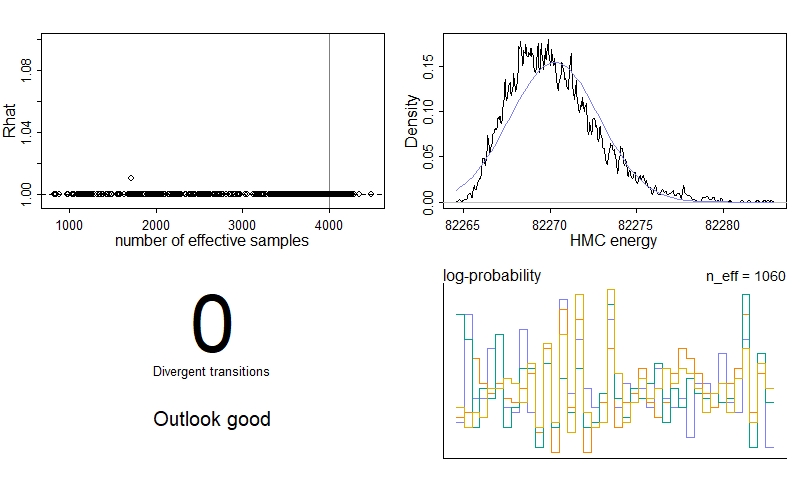
We see no divergent transitions, which is good! The number of effective samples, n_eff is also pretty good for each parameter. We have had one parameter where the Gelman-Rubin convergence diagnostic Rhat isn’t 1, meaning the chains haven’t quite converged - if you look at the summary table, you’ll see it’s actually y0[2], the initial proportion of plant-only patches. However, the problem isn’t too severe, so we’re just going to ignore it in this example.
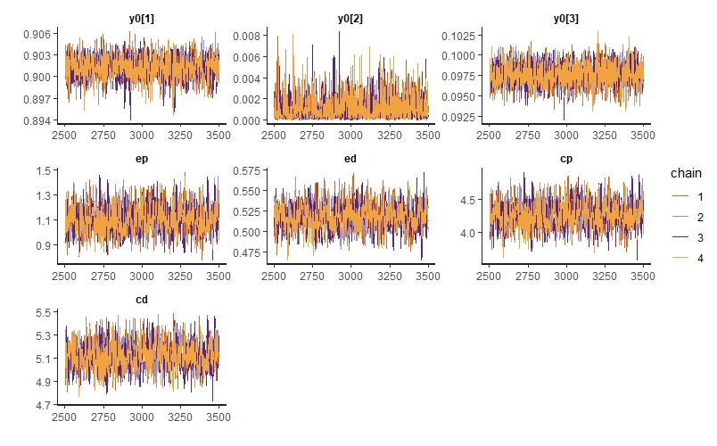
We can also inspect traceplots for our key parameters:
traceplot(m_twosp_mutual, pars=c("y0[1]","y0[2]","y0[3]","ep","ed","cp","cd"))
Now that we’re satisfied with our model’s diagnostics, we’re free to extract the posterior samples:
post <- extract.samples(m_twosp_mutual)
One of the first things we can do is compare our posterior distribution for each of our key parameters with its true value (which we know because we simulated the data!). one way of doing so is with density plots like this:
par(mfrow=c(2,2))
dens(post$ep, main="Plant extinction rate"); abline(v=ep, lty=2)
dens(post$ed, main="Disperser extinction rate"); abline(v=ed, lty=2)
dens(post$cp, main="Plant colonisation rate"); abline(v=cp, lty=2)
dens(post$cd, main="Disperser colonisation rate"); abline(v=cd, lty=2)
par(mfrow=c(1,1))
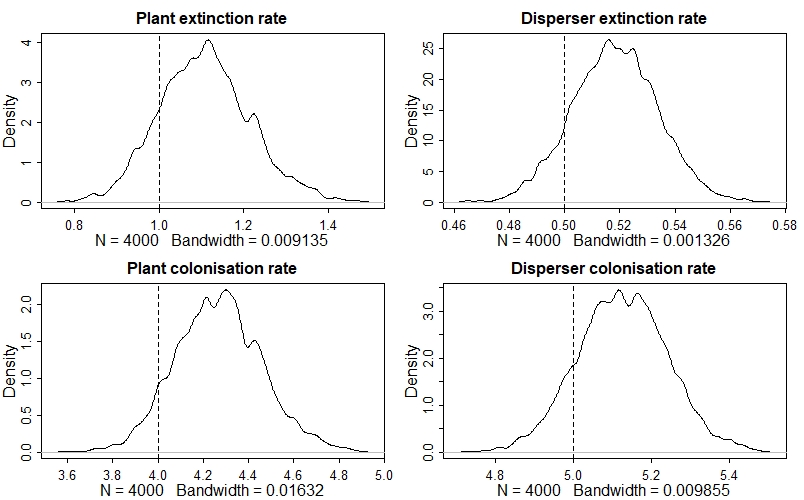
The model has done a good job - all of the dashed vertical lines are contained within their respective posterior distribution!
We can also do this for the initial states:
par(mfrow=c(1,3))
dens(post$y0[,1], main="Initial empty proportion"); abline(v=y0[1], lty=2)
dens(post$y0[,2], main="Initial plant only proportion"); abline(v=y0[2], lty=2)
dens(post$y0[,3], main="Initial both species proportion"); abline(v=y0[3], lty=2)
par(mfrow=c(1,1))
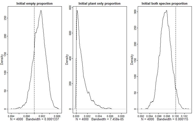
Again, we see that the model has done a good job - if you look at the values on the x-axes, you can see that the estimates are very precise as well.
We can also plot the model’s posterior predictions (as median and compatability intervals) against the observed data, like this:
x_seq <- time

x_sim_mu <- apply(post$n_sim[,,1], 2, median)
x_sim_99CI <- apply(post$n_sim[,,1], 2, HPDI, prob=0.99)
x_sim_95CI <- apply(post$n_sim[,,1], 2, HPDI, prob=0.95)
x_sim_89CI <- apply(post$n_sim[,,1], 2, HPDI, prob=0.89)
x_sim_80CI <- apply(post$n_sim[,,1], 2, HPDI, prob=0.80)
x_sim_70CI <- apply(post$n_sim[,,1], 2, HPDI, prob=0.70)
x_sim_60CI <- apply(post$n_sim[,,1], 2, HPDI, prob=0.60)

y_sim_mu <- apply(post$n_sim[,,2], 2, median)
y_sim_99CI <- apply(post$n_sim[,,2], 2, HPDI, prob=0.99)
y_sim_95CI <- apply(post$n_sim[,,2], 2, HPDI, prob=0.95)
y_sim_89CI <- apply(post$n_sim[,,2], 2, HPDI, prob=0.89)
y_sim_80CI <- apply(post$n_sim[,,2], 2, HPDI, prob=0.80)
y_sim_70CI <- apply(post$n_sim[,,2], 2, HPDI, prob=0.70)
y_sim_60CI <- apply(post$n_sim[,,2], 2, HPDI, prob=0.60)

z_sim_mu <- apply(post$n_sim[,,3], 2, median)
z_sim_99CI <- apply(post$n_sim[,,3], 2, HPDI, prob=0.99)
z_sim_95CI <- apply(post$n_sim[,,3], 2, HPDI, prob=0.95)
z_sim_89CI <- apply(post$n_sim[,,3], 2, HPDI, prob=0.89)
z_sim_80CI <- apply(post$n_sim[,,3], 2, HPDI, prob=0.80)
z_sim_70CI <- apply(post$n_sim[,,3], 2, HPDI, prob=0.70)
z_sim_60CI <- apply(post$n_sim[,,3], 2, HPDI, prob=0.60)

par(mfrow=c(1,3))
plot(NULL, xlim=c(0,10), ylim=c(0,1000), xlab="Time", ylab="Number of patches", main="Empty")
lines(x_seq, x_sim_mu, lwd=2)
shade(x_sim_99CI, x_seq)
shade(x_sim_95CI, x_seq)
shade(x_sim_89CI, x_seq)
shade(x_sim_80CI, x_seq)
shade(x_sim_70CI, x_seq)
shade(x_sim_60CI, x_seq)
points(x = time, y = counts_obs[,1])

plot(NULL, xlim=c(0,10), ylim=c(0,1000), xlab="Time", ylab="Number of patches", main="Plant only")
lines(x_seq, y_sim_mu, lwd=2)
shade(y_sim_99CI, x_seq)
shade(y_sim_95CI, x_seq)
shade(y_sim_89CI, x_seq)
shade(y_sim_80CI, x_seq)
shade(y_sim_70CI, x_seq)
shade(y_sim_60CI, x_seq)
points(x = time, y = counts_obs[,2])

plot(NULL, xlim=c(0,10), ylim=c(0,1000), xlab="Time", ylab="Number of patches", main="Plant & Disperser")
lines(x_seq, z_sim_mu, lwd=2)
shade(z_sim_99CI, x_seq)
shade(z_sim_95CI, x_seq)
shade(z_sim_89CI, x_seq)
shade(z_sim_80CI, x_seq)
shade(z_sim_70CI, x_seq)
shade(z_sim_60CI, x_seq)
points(x = time, y = counts_obs[,3])
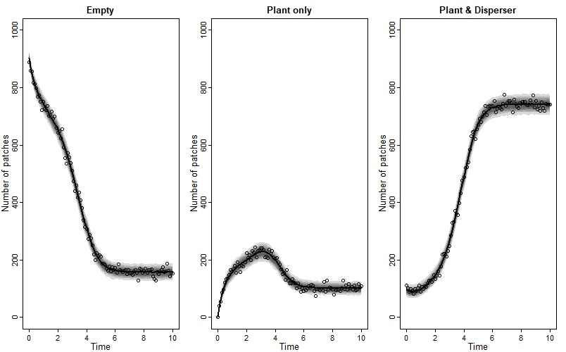
We see a great fit!
Comments