
Classic ecological models in Stan: exponential and logistic growth
In this post, I cover how to fit two simple models of population growth using Stan: exponential growth, and logistic growth. I also cover how to use R to simulate data to fit these models to.
Introduction, and an idea for a series
I recently decided that I’d like to learn more about Stan, and especially about how to fit different kinds of models - more than just the glm’s which I’ve been learning about since undergrad. I also enjoy learning about theoretical ecology, and thought it would be cool to combine these two interests - and hopefully help some people along the way! As a result, I decided it would be cool to learn how to fit some classic ecological models using Stan, and to share my learning in these posts.
I was also inspired by a couple of examples of people doing this already - this paper on fitting the SIR disease transmission model by Léo Grinsztajn and colleagues made me realise just how versatile Stan could be, and was a major contributor towards me deciding to learn it. The second example is the Lotka-Volterra predator-prey model as demonstrated by Richard McElreath in Statistical Rethinking - the impact of predators on prey populations is something I’ve been interested in for years (ever since an essay assignment I particularly enjoyed as an undergrad), so it was very exciting to learn that I could fit models like this in Stan.
I don’t really have a definition for what constitutes a ‘classic’ model - I thought I’d just start off with some models I was taught about as an undergrad or have read about in books, and follow my interests from there. If there’s a model that you’d like to see featured, then feel free to drop me a message - there’s no guarantee that I’ll cover it (not least because I may be unable to code it…), but I’ll do my best!
Acknowledgements and other resources
I learned a lot about modeling from the book a biologist’s guide to mathematical modeling in ecology and evolution by Sarah Otto and Troy Day, and it was one of the main resources I used when writing this post.
I also learned a great deal from the classic book theoretical ecology: principles and applications (3rd ed.), edited by Robert May and Angela McLean - the chapter on single-species dynamics by Tim Coulson and Charles Godfray is most relevant here, but the whole book is fantastic and well worth reading.
As for my knowledge about Stan, I mainly learned from the book and online course Statistical Rethinking by Richard McElreath, and also found Michael Betancourt’s introduction to Stan to be very useful.
For more differential-equation-specific Stan knowledge, I mostly learned from the Stan manual, supplemented by this post about (relatively) recent changes to the ODE interface and this tutorial by Mikhail Popov.
Disclaimer
As I am writing this post largely as a way of learning about the material, I would not be surprised if it contains mistakes. Please bear this in mind when reading it, and remember that any use of the model etc. is at your own risk.
If you do happen to spot any mistakes, I’d be very grateful if you would let me know in the comments below or by email (my contact details are in the sidebar) so that I can correct them!
Exponential growth
Introducing the model
Organisms are born, and then they die. From these two facts, we can build the most simple model of population growth:
\[\frac{dn}{dt} = bn(t) - dn(t)\]where the population size is $n$, time is $t$, the birth rate is $b$, and the death rate is $d$. This model is an ordinary differential equation (ODE), which describes how the derivative $(\frac{dn}{dt}$: the tiny change in population size n that occurs over each tiny change in time t) changes, as a function of the population size itself.
We can actually make this model even simpler, by replacing the birth and death rates with a single parameter $r$ which is just the difference between them:
\[r = b-d\]This means that $r$ represents the population’s per-capita rate of change. We can replace $b$ and $d$ with $r$ in our equation, making it:
\[\frac{dn}{dt} = rn(t)\]Our goal is now going to be to infer $r$ from the data. But first, we have to simulate the data!
Simulating the data in R
First, let’s a couple of packages and setting the seed for the random number generator:
library(rethinking)
library(deSolve)
set.seed(555)
We’re going to start off by simulating the underlying exponential growth process. The first thing to do is to define a function which takes in values for the intial state y0 and rate of change r, and spits out the derivative dn.dt for each time step:
exp_growth <- function(times,y,parms){
  dn.dt <- r[1]*y[1]
  return(list(dn.dt))
}
The next step is to pick some values for the parameters, as well as a time sequence to simulate for. We’re going to assume that our rate of change r is constant at all points in time:
r <- 0.5 # Rate of change
y0 <- 1 # Initial state
time <- seq(0,10,by=0.1) # Time sequence
After this, we can simulate our true population size over time by using the ode function in the deSolve package to obtain the population size at each point in time:
n_true <- ode(y=y0, times=time, func = exp_growth, parms = r)
We can plot it like so:
plot(time, n_true[,2], ylab="Population size")
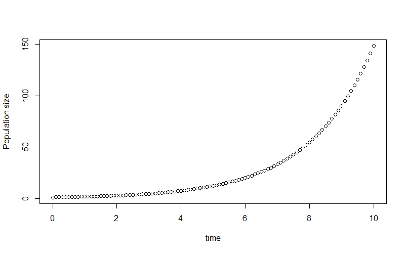
This allows us to see the classic exponential growth curve.
Now that we’ve simulated our true population growth, we’re going to simulate the observation process. I’m going to simulate the observed population size, n_obs, at each time-step using a $Poisson$ distribution where $\lambda$ is the true population size at a given time. This has a couple of good features: it ensures that the observed population size is always a positive integer (or zero), and it also means that the variation in observed values is greater when the population size is greater - which represents a scenario where measurement error is greater when the population is large. We can simulate and plot the observed data like this:
n_obs <- rpois(n = length(time),
               lambda = n_true[,2])
plot(n_obs ~ time, xlab="Time", ylab="Observed population size")
points(time, n_true[,2], type="l", lwd=2)
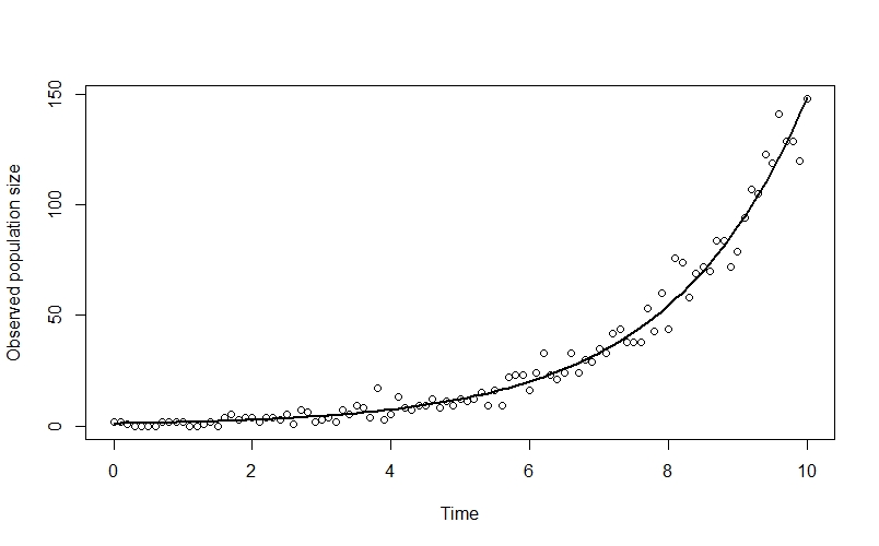
Here I’ve plotted the true population trend in black, so you can see the way that the observed datapoints deviate from the line.
Now that we’ve simulated our data, we can prepare a data list for Stan. This requires some slight creativity due to the way that Stan indexes time steps (starting at 1, not at zero) - meaning we have to separate initial state bits y0_obs and t0, and subtract the first element from y and ts. We also have to subtract 1 from our time index n_times. The code looks like this:
dlist <- list(
  n_times = length(time)-1L, # Number of timesteps
  y0_obs = n_obs[1], # Observed initial state
  y = n_obs[-1], # Observed data
  t0 = 0, # Initial timestep
  ts = time[-1] # Timesteps
)
We can now go on to code our model!
Coding the model in Stan
Here is the full model:
functions{
  vector exp_growth(real t, // Time
                    vector y, // State
                    real r){ // r parameter
    vector[1] dndt;
    dndt[1] = r*y[1];
    return dndt;
  }
}
data {
  int<lower=1> n_times; // Number of time steps minus one
  array[n_times] int y; // Observed data, minus initial state
  int<lower=0> y0_obs; // Observed initial state
  real t0; // First time step
  array[n_times] real ts; // Time steps
}
parameters {
  vector[1] y0; // Initial state
  real r; // Per-capita rate of population change
}
transformed parameters{
    // ODE solver
  vector[1] lambda[n_times] = ode_rk45(exp_growth, y0, t0, ts, r);
}
model {
  // Priors
  r ~ normal(0, 1);
  y0 ~ exponential(1);

  // Likelihood
  y0_obs ~ poisson(y0[1]);
  for (t in 1:n_times) {
    y[t] ~ poisson(lambda[t]);
  }
}
generated quantities{
  array[n_times+1] int n_sim;
  n_sim[1] = poisson_rng(y0[1]);
  for(t in 1:n_times){
    n_sim[t+1] = poisson_rng(lambda[t,1]);
  }
}
Now let’s go through it step-by-step!
The functions block
functions{
  vector exp_growth(real t, // Time
                    vector y, // State
                    real r){ // r parameter
    vector[1] dndt;
    dndt[1] = r*y[1];
    return dndt;
  }
}
The functions block is where a lot of the action happens for ODE-based models like ours, so it’s worth spending a little bit of time on.
Apparently the way that ODE’s work in Stan was changed relatively recently, however it seems to me that the general idea hasn’t changed - we write a function for our ODE in the functions block, and then give this function to the ODE solver later on in our model.
There are essentially two parts to our function. The first bit, from left to right, tells the function that we want our output as a vector (this is the only option allowed), that our function is called exp_growth (you can name it anything you like), and that our function has three inputs: real t, which is a time; vector y, which is the system’s state; and real r which is our ODE’s single parameter $r$. We could add more inputs if we had more parameters - this is exactly what we’ll do in the logistic growth model later on.
The second part of our function is where we actually code the ODE. We first have to make a vector, which I’ve called dndt, to store our time derivatives (i.e., our output). We then get to do the interesting bit, which is to actually code our differential equation: dndt[1] = r*y[1];. Finally, we just ask the function to return our output, dndt.
The data block
data {
  int<lower=1> n_times; // Number of time steps minus one
  array[n_times] int y; // Observed data, minus initial state
  int<lower=0> y0_obs; // Observed initial state
  real t0; // First time step
  array[n_times] real ts; // Time steps
}
In this block we tell Stan about our data. Remember that when we were making dlist ealier on, we had to separate the initial state from the rest of the time series - we have to do the same thing in this block.
We first have n_times, which tells Stan how many time steps are after the initial state.
We then have our observed data y, as well as our observed initial state y0_obs.
After this, we have our initial time step t0 followed by an array our time steps ts.
The parameters block
parameters {
  vector[1] y0; // Initial state
  real r; // Per-capita rate of population change
}
Here we tell Stan about the parameters of our model - the populaton’s initial state y0 and the per-capita rate of change r.
The transformed parameters block
transformed parameters{
    // ODE solver
  vector[1] lambda[n_times] = ode_rk45(exp_growth, y0, t0, ts, r);
}
This block contains the ODE solver - the function that solves the ODE, giving us an equation for the population size $n$ at any point in time.
In this example we’re using the ode_rk45 solver, which is often a good sover to start with. You can find out about the other solvers which Stan provides in the Stan functions reference. We need to give the solver our function exp_growth that we wrote in the functions block, the initial state parameter y0, the first timestep t0 and the rest of the times ts, and our model’s parameters - in this case, it’s just r.
This code needs to go in the transformed parameters block, rather than the model block, so that lambda is available to the generated quantities block later on.
The model block
model {
  // Priors
  r ~ normal(0, 1);
  y0 ~ exponential(1);

  // Observation model
  y0_obs ~ poisson(y0[1]);
  for (t in 1:n_times) {
    y[t] ~ poisson(lambda[t]);
  }
}
In this block, we start of by specifying priors for the parameters in our model. I’ve assumed a $Normal(0, 1)$ prior for $r$, which is probably not a great choice since we are probably going to know that the population is increasing over time (meaning $r$ must be positive) - but it’ll do for this example. I’ve given the initial state y0 an $exponential(1)$ prior, since we know for certain it has to be positive (it can’t be negative because a negative population size makes no sense, and if it’s zero then we’ll only ever observe zero individuals so we’ll hopefully notice pretty quickly!) and it’s also likely to be small.
After the priors, we have the section of the model which deals with the observation process. The first line models the initial state, and the for loop deals with all of the subsequent timesteps.
The generated quantities block
generated quantities{
  array[n_times+1] int n_sim;
  n_sim[1] = poisson_rng(y0[1]);
  for(t in 1:n_times){
    n_sim[t+1] = poisson_rng(lambda[t,1]);
  }
}
In this block, we’re going to perform posterior predictive simulations - at each sampling iteration, we’re going to simulate a population time series n_sim using the lambda values from that iteration and the poisson_rng random number generator for the Poisson distribution. Later on, we’re going to compare these simulated values against the observed data to evaluate the model’s fit.
Actually coding this block is a little bit of a pain, mostly due to indexing - because we separated the initial time step in the other parts of the model, we have to compute the first value of n_sim using our initial state parameter y0[1], and then compute all of the other n_sim values using the appropriate lambda value. In order to make the indexes match up in the correct place, we have to define n_sim as having n_times+1 values and then index it as n_sim[t+1] in the for loop.
Running the model and exploring the output
We first need to save our model as a .stan file somewhere - when that’s done, we can run the model using the cstan function in the rethinking package:
m_exp <- cstan(file = "C:/Stan_code/exponential_growth.stan",
               data = dlist,
               chains = 4,
               cores = 4,
               warmup = 1500,
               iter = 2500,
               seed = 654)
The model will now compile and sample - why not help to classify some of my camera trap photos while it does so? ![]() When it’s done, we can inspect the
When it’s done, we can inspect the precis summary table - I’m going to just show the first few rows here, but the real thing is quite long:
precis(m_exp, depth =3)
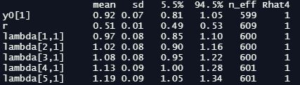
As you can see, we have our initial state parameter y0 and our rate of change r at the top. We then have the lambda values for the 100 timesteps after the initial step, followed (in the non-truncated version you’ll see if you run the code) by the 101 n_sim values produced by the generated quantities block. At this point we’re particularly interested in our effective sample size n_eff and Gelman-Rubin convergence diagnostic Rhat4 - we want the first to be a reasonably high number (ours look fine here), and we want the latter to equal one. It’s also a good idea to inspect traceplots for our key parameters at this point:
traceplot(m_exp, pars=c("y0[1]","r"))
Now we see that the model has sampled successfully, we can figure out whether it did a good job fitting the data. The first thing that we can do (since we simulated the data and know the true parameter values!) is to see how well the model estimated the per-capita rate of change, $r$ - as this is the parameter that we’re really interested in:
dens(post$r)
abline(v=r, lty=2)
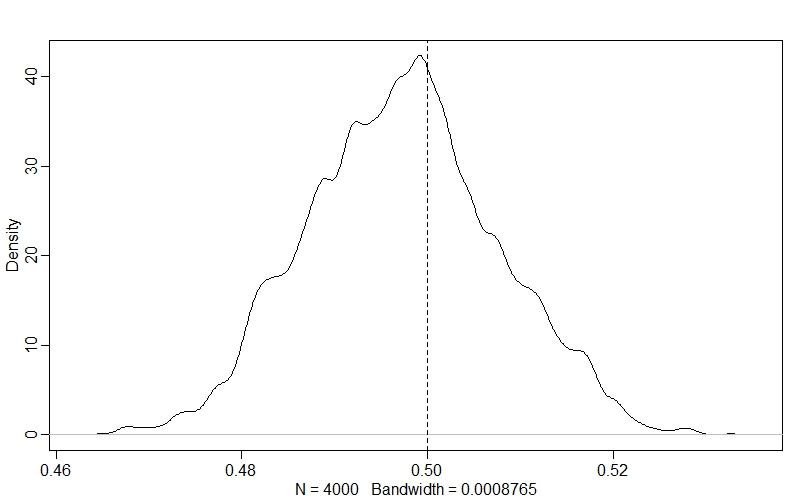
The model has really hit the nail on the head here - the true value for $r$ is right in the middle of our posterior distribution!
We can also plot the model’s posterior predictions against the raw data, like this:
x_seq <- seq(0,10,0.1)

n_sim_mu <- apply(post$n_sim, 2, median)
n_sim_99CI <- apply(post$n_sim, 2, HPDI, prob=0.99)
n_sim_95CI <- apply(post$n_sim, 2, HPDI, prob=0.95)
n_sim_89CI <- apply(post$n_sim, 2, HPDI, prob=0.89)
n_sim_80CI <- apply(post$n_sim, 2, HPDI, prob=0.80)
n_sim_70CI <- apply(post$n_sim, 2, HPDI, prob=0.70)
n_sim_60CI <- apply(post$n_sim, 2, HPDI, prob=0.60)

plot(NULL, xlim=c(0,10), ylim=c(0,200), xlab="Time", ylab="Population")
lines(x_seq, n_sim_mu, lwd=2)
shade(n_sim_99CI, x_seq)
shade(n_sim_95CI, x_seq)
shade(n_sim_89CI, x_seq)
shade(n_sim_80CI, x_seq)
shade(n_sim_70CI, x_seq)
shade(n_sim_60CI, x_seq)

points(x_seq, n_obs)
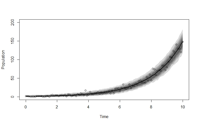
The fit looks very good!
Logistic growth
Introducing the model
Populations can’t just grow exponentially forever - sooner or later, intraspecific competition, limited resources and other factors prevent the population from growing further.
To model this idea, we can extend the exponential growth model by introducing a carrying capacity ($K$), which is the maximum size which our population will reach. We can include $K$ in our model n such a way that when the population size equals the carrying capacity, $\frac{dn}{dt}$ will equal zero and the population will cease to grow any further. This means that the rate of population growth is density dependent - as the population gets larger, the rate of increase slows. The model looks like this:
\[\frac{dn}{dt} = rn(t)\left(1-\frac{n(t)}{K}\right)\]You can actually derive this specific equation by assuming that $r$ declines linearly as the population size increases - Otto and Day cover this in their book, so I’m not going to go into it here.
Simulating the data in R
Simulating data for logistic growth is actually very similar to the process we carried out for exponential growth, so rather than going through it step-by-step I’m just going to present the whole simulation code in one go. The main change is that we’ve changed our function to the equation for logistic growth, and we’ve added the parameter for the carrying capacity K in the appropriate places:
# Function for logistic growth
logistic_growth <- function(times,y,parms){
dn.dt <- r[1]*y[1]*(1-(y[1]/K))
return(list(dn.dt))
}
# Values for parameters and time sequence
r <- 0.5 # Per-capita rate of change
K <- 50 # Carrying capacity
y0 <- 1 # Initial state
time <- seq(0,25,by=0.1) # Time sequence
# Simulate true population size
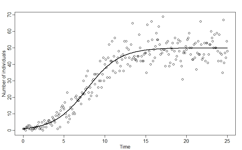
n_true <- ode(y=y0, times=time, func = logistic_growth, parms = c(r,K))
plot(time, n_true[,2])
# Simulate observation process
n_obs <- rpois(n = length(time),
lambda = n_true[,2])
# Plot observed data and true line
plot(n_obs ~ time, xlab="Time", ylab="Number of individuals")
points(time, n_true[,2], type="l", lwd=2)
# Make a data list for Stan
dlist <- list(
n_times = length(time)-1L,
y0_obs = n_obs[1],
y = n_obs[-1],
t0 = 0,
ts = time[-1]
)
Plotting the observed data along with n_true, we can see how our datapoints fall around the classic “S-curve”:
Coding the model in Stan
Now we can code the model in Stan. Here is the full model:
functions{
  vector logistic_growth(real t,
                    vector y,
                    real r,
                    real K){
    vector[1] dndt;
    dndt[1] = r*y[1]*(1-(y[1]/K));
    return dndt;
  }
}
data {
  int<lower=1> n_times;
  array[n_times] int y;
  int<lower=0> y0_obs;
  real t0;
  array[n_times] real ts;
}
parameters {
  vector[1] y0;
  real r;
  real K;
}
transformed parameters{
    // ODE solver
  vector[1] lambda[n_times] = ode_rk45(logistic_growth, y0, t0, ts, r, K);
}
model {
  // Priors
  r ~ normal(0, 1);
  y0 ~ exponential(1);
  K ~ exponential(0.05);

  // Likelihood
  y0_obs ~ poisson(y0[1]);
  for (t in 1:n_times) {
    y[t] ~ poisson(lambda[t]);
  }
}
generated quantities{
  array[n_times+1] int n_sim;
  n_sim[1] = poisson_rng(y0[1]);
  for(t in 1:n_times){
    n_sim[t+1] = poisson_rng(lambda[t,1]);
  }
}
It actually looks really similar to the exponential growth model - there are only a few minor changes to the functions, parameters, transformed parameters, and model blocks. Let’s go through these step by step:
The functions block
This is the bit with the most changes, but even here they’re pretty minor - we’ve just added a slot for our carrying capacity K in our function, and changed the equation to the one for the logistic growth model.
The data block
No changes here!
The parameters block
In this block, we’ve just added the parameter K for the carrying capacity.
The transformed parameters block
The only thing new here is adding K to the ode_rk45 function.
The model block
The only thing we’ve changed here is adding a prior for the carrying capacity, K. There are probably better choices than the $exponential(0.05)$ prior I’ve got here, but my choice does at least constrain K to be positive.
The generated quantities block
No changes here!
Running the model and exploring the output
We can run the model and explore the output using almost the same code as we used for the exponential growth model - we just have to substitute in the new model name where appropriate, and slightly alter the scale at which we’re plotting the data due to the different time and population ranges we’re dealing with. Here is all of the code to run the model, check the summary table and traceplots, and plot our posterior predictions against the observed data:
# Run the model
m_log <- cstan(file = "C:/Stan_code/logistic_growth.stan",
data = dlist,
chains = 4,
cores = 4,
warmup = 1500,
iter = 2500,
seed = 543)
# Summary table
precis(m_log, depth =3)
# Traceplots for key parameters
traceplot(m_log, pars=c("y0[1]","r","K"))
# Extract posterior samples
post <- extract.samples(m_log)
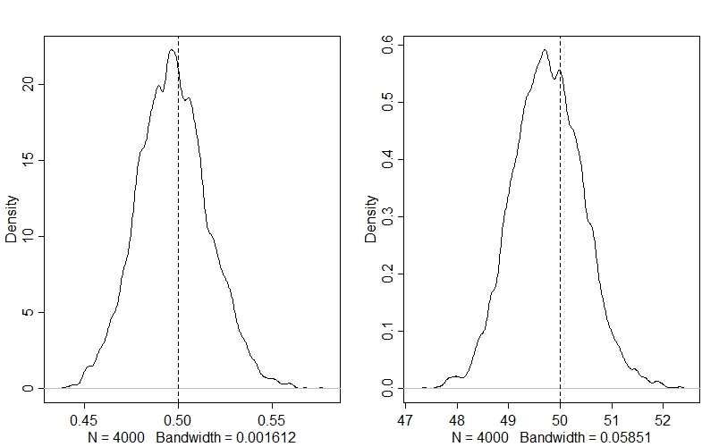
# Density plots for key parameters - vertical lines for true values
par(mfrow=c(1,2)
dens(post$r)
abline(v=r,lty=2)
dens(post$K)
abline(v=K, lty=2)
par(mfrow=c(1,1)
# Posterior predictive plot
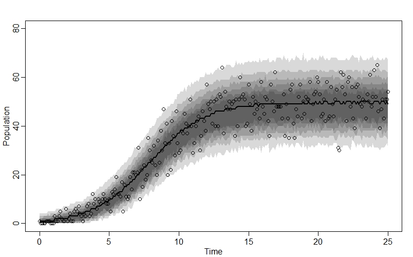
x_seq <- seq(0,25,0.1)
# Calculate mean and compatability intervals for n_sim
n_sim_mu <- apply(post$n_sim, 2, median)
n_sim_99CI <- apply(post$n_sim, 2, HPDI, prob=0.99)
n_sim_95CI <- apply(post$n_sim, 2, HPDI, prob=0.95)
n_sim_89CI <- apply(post$n_sim, 2, HPDI, prob=0.89)
n_sim_80CI <- apply(post$n_sim, 2, HPDI, prob=0.80)
n_sim_70CI <- apply(post$n_sim, 2, HPDI, prob=0.70)
n_sim_60CI <- apply(post$n_sim, 2, HPDI, prob=0.60)
# Make the plot
plot(NULL, xlim=c(0,25), ylim=c(0,80), xlab="Time", ylab="Population")
lines(x_seq, n_sim_mu, lwd=2)
shade(n_sim_99CI, x_seq)
shade(n_sim_95CI, x_seq)
shade(n_sim_89CI, x_seq)
shade(n_sim_80CI, x_seq)
shade(n_sim_70CI, x_seq)
shade(n_sim_60CI, x_seq)
points(x_seq, n_obs) # Add points for raw data
Looking at our values for $r$ (left) and $K$ (right), we can see that the model has accurately estimated both parameters:
And when we plot the model’s posterior predictions against the raw data, we see a great fit:
Comments