
An occupancy model with a Gaussian process for spatial autocorrelation in Stan
In this post I walk through an occupancy model which uses a Gaussian process to model spatial autocorrelation. The model is coded in Stan. I start off with a brief overview of occupancy models and Gaussian process regression. I then walk through how to simulate a dataset from the assumed data-generating process in R, and then explain the model and Stan code step-by-step. Finally, I look at some of the interesting things we can do once we have the posterior distribution.
Acknowledgements and other resources
I used several resources when writing this post. In particular, the majority of my knowledge about Bayesian statistics, Stan, and Gaussian processes comes from Richard McElreath’s fantastic book and lecture series Statistical Rethinking. The whole course is available for free online, I highly recommend you check out the most recent version here. I also learned a lot about Stan from Michael Betancourt’s excellent case studies, in particular the introduction to Stan. I learned about how to marginalise out the discrete occupancy state parameters from Maxwell B. Joseph’s tutorial, and the supplement of this paper by Allan Clark and Res Altwegg - my understanding mainly comes from the former, my code from the latter. Some of the other key resources which I used to learn about about occupancy models are the classic book by MacKenzie et al. and this paper by Joe Northrup and Brian Gerber. I’d also like to thank the Conservation Ecology Group at Durham University, as this post was inspired by a talk I gave at one of their lab group meetings a few months ago.
An important note
This post should be considered a work in progress - I greatly appreciate any feedback which I can implement to improve it, particularly if you spot any mistakes!
Introduction
Occupancy models
Occupancy models are used to study the patterns and drivers of species occurrence. They are very commonly used for camera trap data, which is why I got interested in them in the first place. One of their key characteristics is that they deal with imperfect detection - the chance that a species which is present at a site may remain undetected. In this section, I’ll walk through a standard single-season occupancy model - I follow the model notation from Northrup and Gerber pretty closely here. We’ll expand the model to include spatial autocorrelation in the next section.
Imagine that we have a bunch of sites dotted about the landscape. The state ($z$) of a site (indexed $i$) is either occupied (1) or unoccupied (0), and the probability that it is occupied is called the occupancy probability ($\psi$). We can write this as:
\[z_{i} \sim Bernoulli(\psi_{i})\]We assume that a site stays in one state (occupied or not) for the duration of the study, i.e. that there is a single season. You can also get multi-season or dynamic occupancy models which assume that the state may change, but I’m not going to cover those here.
We’re often interested in modelling $\psi$ as a function of one or more covariates, for instance because we want to know the effect of some environmental variable on occupancy. It’s important to note that it is very important to consider the purpose of the model (inference or prediction) when deciding on which covariates to put in the model - this is covered by my recent preprint. We can add covariates in a standard logistic regression format, for example for a single covariate $X$:
\[logit(\psi_{i}) = ln(\frac{\psi}{1-\psi}) = \alpha + \beta_{X}X_{i}\]Now comes the bit where we account for imperfect detection. We visit each site multiple ($v_{i}$) times and record whether we observe the species on each visit. The observed data at each site ($y_{i}$) can then be modelled as:
\[y_{i} \sim Binomial(v_{i}, \mu_{i})\\ \mu_{i} = p_{i}z_{i}\]In the second line, $z_{i}$ is the true occupancy state and $p_i$ is the probability of detection. Therefore, if a species is absent from a site is is never detected, and if it is present it is detected on each visit with probability $p$. We can also make the detection probability a function of covariates, for instance:
\[logit(p_{i}) = ln(\frac{p}{1-p}) = \alpha_{det} + \beta_{W}W_{i}\]It’s also pretty common to see models where detection probability is allowed to be different on each visit and you have a time-varying covariate - this would be great for situations in which the probability we detect a species on a visit varies due to factors such as weather. The only thing we need to change is the indexing - for instance, we could now have $W_{i,j}$ for the value of $W$ at site $i$ on visit $j$. This is what I do in the example model later on.
Taking everything we’ve got so far, the full model with priors would look like:
\[y_{i} \sim Binomial(v_{i}, \mu_{i})\\ \mu_{i} = p_{i}z_{i} \\ z_{i} \sim Bernoulli(\psi_{i}) \\ logit(\psi_{i}) = ln(\frac{\psi}{1-\psi}) = \alpha + \beta_{X}X_{i} \\ logit(p_{i}) = ln(\frac{p}{1-p}) = \alpha_{det} + \beta_{W}W_{i} \\ \beta_{X} \sim Normal(0,1) \\ \beta_{W} \sim Normal(0,1) \\ \alpha \sim Normal(0,1) \\ \alpha_{det} \sim Normal(0, 0.5)\]You’d want to pick the specific priors for your problem at hand by doing some prior predictive simulations, which we’ll do for our example later on.
Now, it’s time to expand our occupancy model to account for spatial autocorrelation!
Spatial autocorrelation and Gaussian process regression
The occupancy model above assumes that the occupancy probability of our sites is independent, regardless of where they are situated in space. However, in many instances this is unlikely to be the case - sites which are closer together tend to be more similar than sites which are further apart. This phenomenon is called spatial autocorrelation.
There are a variety of ways that we could include this spatial autocorrelation in our model. One really cool way is to use Gaussian process regression.
The theory behind Gaussian process regression is already covered by Statistical Rethinking, as well as this case study and the Stan Users’ guide. For this reason, I’m just going to give a quick overview here so that our extensions to the occupancy model make sense.
Remember that the essential idea is that sites which are closer tend to be more similar. A natural way to express this idea is by having a function to link the covariance between a pair of sites (we’ll index these $i$ and $j$) to the distance between them. This function is usually called a kernel function, and one example is:
\[K_{i,j} = \eta^2exp(-\rho^2D^2_{i,j})\]Where $K_{i,j}$ is the covariance between sites $i$ and $j$, $\eta^2$ is the maximum covariance between sites, $\rho^2$ is the rate that covariance declines with distance, and $D^2_{i,j}$ is the (squared) distance between sites $i$ and $j$. Because we have more than one pair of sites, we’re going to feed in a distance matrix and end up with a covariance matrix.
We now want to turn this covariance matrix into something that we can use in our linear model for occupancy probability - we want some kind of varying intercept. One way of doing this is to have an average intercept across all sites ($\bar{k}$) and then a site-specific offset ($k_{i}$) like so:
\[logit(\psi_{i}) = ln(\frac{\psi}{1-\psi}) = \bar{k} + k_{i} + \beta_{X}X_{i} \\\]Notice that what we’ve done is replace the intercept ($\alpha$) from the model we saw earlier with $\bar{k}$ and $k_{i}$. We’ve still got the covariate $X$ as before. The final thing we need to do is connect our site-level offset $k_{i}$ back to the kernel function. We can do this using the multivariate normal distribution, like this:
\[\begin{pmatrix}k_{1} \\ k_{2} \\ \vdots \\ k_{i} \end{pmatrix} \sim MVNormal\left(\begin{pmatrix}0\\0\\0\\0\end{pmatrix}, \textbf{K}\right)\]You can see the covariance matrix $\textbf{K}$ formed from all of the combinations of $K{i,j}$ on the right. The mean of the multivariate normal distribution is filled with zeroes because we already have $\bar{k}$ in the model above.
The only thing left to do is add some priors for the new parameters - with the priors included, the whole model looks like:
\[y_{i} \sim Binomial(v_{i}, \mu_{i})\\ \mu_{i} = p_{i}z_{i} \\ z_{i} \sim Bernoulli(\psi_{i}) \\ logit(\psi_{i}) = ln(\frac{\psi}{1-\psi}) = \bar{k} + k_{i} + \beta_{X}X_{i} \\ \begin{pmatrix}k_{1} \\ k_{2} \\ \vdots \\ k_{i} \end{pmatrix} \sim MVNormal\left(\begin{pmatrix}0\\0\\0\\0\end{pmatrix}, \textbf{K}\right) \\ K_{i,j} = \eta^2exp(-\rho^2D^2_{i,j}) \\ logit(p_{i}) = ln(\frac{p}{1-p}) = \alpha_{det} + \beta_{W}W_{i} \\ \beta_{X}, \beta_{W} \sim Normal(0,1) \\ \alpha_{det} \sim Normal(0, 0.5)\\ \bar{k} \sim Normal(0, 0.2) \\ \eta^2, \rho^2 \sim Exponential(1)\]Again, prior predictive simulations were used to help choose the priors - I cover how to do these below.
Simulating from the data-generating process in R
A really good way to help develop a model is to think about the process which could have produced the data, and then make a simulation of this process. We can then fit the model to these simulated data, which is a great way of identifying and fixing any issues with our model before we fit it to real data!
In this section, we’ll go through the code I used to simulate the data.
Let’s start by loading a couple of packages that we’ll need:
library(rethinking)
library(MASS)
Now, let’s set up some basic parameters for the simulation - we’ll go for 100 sites, with each site surveyed somewhere from 14 to 21 times. We’ll also set a seed for R’s random number generator, so that you can replicate my results exactly:
sites <- 100
surveys <- sample(14:21, size=sites, replace=TRUE)
set.seed(1234)
Now we’re going to generate a random set of x and y coordinates for each site, showing where it is situated in our study region. We’re then going to use these coordinates to make a distance matrix, which contains the distance between each pair of sites:
x <- runif(sites, 0, 10) # x coordinate
y <- runif(sites, 0, 10) # y coordinate

coords <- as.data.frame(cbind(x,y))

# Make distance matrix from coordinates
dmat <- dist(coords, diag=T, upper=T)
dmat <- as.matrix(dmat)

dmat2 <- dmat^2 # Squared distances
Now that we’ve got our distance matrix, we need to code the function that calculates the covariance between each pair of sites from the distance between them. Remember that our kernel function is:
\[K_{i,j} = \eta^2exp(-\rho^2D^2_{i,j})\]with definitions as above. We’re going to pick some values for $\eta^2$ and $\rho^2$ and then generate the covariance matrix:
eta2 <- 0.8
rho2 <- 0.5
covmat <- eta2*exp(-rho2*dmat2) # Max value should be eta2 on the diagonals
You can visualise how our choice of values affects the kernel function by plotting covariance against distance. It’s also helpful here to plot the distribution of distances between sites, to see how many pairs will have each amount of covariance:
par(mfrow=c(1,2))
curve(eta2*exp(-rho2*x^2),from=0, to=10, lty=1, xlab="Distance", ylab="Covariance") # Visualise covariance (y) vs distance (x)
dens(as.vector(dmat), xlab="Distance") # Visualise the distances between sites as well
par(mfrow=c(1,1))
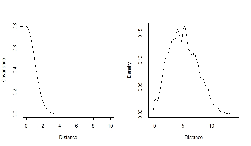
You can use this code to play around with the $\eta^2$ and $\rho^2$ values to see how they affect the way that covariance declines with distance.
Now that we have our covariance matrix, we want to use it to generate a varying intercept for the occupancy probability. This means that sites which are closer together tend to have a more similar occupancy probability. We do this using the multivariate normal distribution with the mvrnorm function from the MASS package:
z <- rep(0, nrow(covmat))

varint <- mvrnorm(n = 1,
                  mu = z,
                  Sigma = covmat)
varint <- as.numeric(varint)
Note that we’re ignoring $\bar{k}$ here and making the mean in mvnorm zero, which is the same as assuming that $\bar{k}$ is equal to zero.
Now we’re going to add two covariates for the occupancy probability: $X$, which is our focal variable (i.e., we’re interested in the effect of $X$ on $\psi$ ) and $M$, which is a confounding variable. We will assume that the variables are related as shown in this DAG:
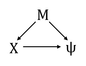
The consequence is that if we want to estimate the effect of $X$ on $\psi$, we need to condition on $M$ in our occupancy sub-model. We will also include a covariate $W_{t}$ for the detection probability. We’re giving this covariate the subscript $t$ because it is time-varying, meaning that it has a different value for each survey of the site.
Let’s code up the covariates, effect sizes ($\beta_{X}, \beta_{M},$ and $\beta_{MX}$), and the true occupancy and detection probabilities:
# True effect sizes:
betax <- 1.0 # Effect of x on psi
betam <- -0.8 # Effect of m on psi
betamx <- 0.5 # Effect of m on x

# Variables
m <- rnorm(sites, 0, 1)
x <- rnorm(sites, betamx*m, 1)

# True occupancy probability at each site
psi <- inv_logit(varint + betax*x + betam*m)

# Covariate for detection probability
w <- matrix(NA, nrow=sites, ncol=max(surveys))

for(i in 1:sites){
  for(k in 1:surveys[i]){
    w[i,k] <- rnorm(1,0,1)
  }
}

# True detection probability
alphadet <- -0.1 #
betadet <- 0.4 #

pdet <- matrix(NA, nrow=sites, ncol=max(surveys))

for(i in 1:sites){
  for(k in 1:surveys[i]){
    pdet[i,k] <- inv_logit(alphadet + betadet*w[i,k])
  }
}
Now we’re ready to populate our simulated landscape and conduct our simulated surveys! Let’s simulate the true occupancy state (1 = occupied, 0 = unoccupied) for each site, and then simulate the observed detection history for each site:
# True occupancy state
z <- rep(NA, length=sites)
for(i in 1:sites){
  z[i] <- rbinom(1,1,psi[i])
}

# Observed detection history
y <- matrix(NA, nrow=sites, ncol=max(surveys))
for(i in 1:sites){
  for(k in 1:surveys[i]){
    y[i,k] <- rbinom(1,1,pdet[i,k]*z[i])
  }
}
Finally, let’s get the data ready for Stan.
As Stan can’t deal with the NA values in visits which did not occur (e.g., where a site was surveyed 17 times, the final 4 surveys will be NA), we have to replace them with a number - the specific number doesn’t really matter, because Stan should never access the values in its calculations. I prefer to use a ridiculous number like -9999 because then if Stan does access the number somehow, it should result in an error which is relatively easy to detect.
We can then make the data list for Stan to use. This includes the observed data y, the covariates x, m and w, the distance matrix dmat, the number of sites nsites, the number of surveys at each site V and the maximum number of visits made to a site, N_maxvisits:
y[is.na(y)] <- -9999
mode(y) <- "integer"

w[is.na(w)] <- -9999

# Data list for Stan
dlist <- list(
  nsites = as.integer(sites),
  N_maxvisits = as.integer(max(surveys)),
  V = surveys,
  y = y,
  x = x,
  m = m,
  w = w,
  dmat = dmat
)
Prior predictive simulations
As I mentioned earlier, we’re going to use prior predictive simulations to help choose our priors for the model. There are two main sets of parameters that we need to think about here: the effect sizes and intercepts for the occupancy and detection linear models ($\beta_{X}, \beta_{M},\alpha_{det},\beta_{det}$) and the parameters for the Gaussian process ($\eta^2$ and $\rho^2$).
Let’s start with the first set of parameters - the effect sizes and intercepts. Let’s think about the detection submodel to start with. Remember that the relevant bit of our model is:
\[logit(p_{i}) = ln(\frac{p}{1-p}) = \alpha_{det} + \beta_{W}W_{i} \\ \alpha_{det} \sim Normal(?,?) \\ \beta_{W} \sim ~Normal(?,?)\]I’ve suggested that we use normal prior distributions for our two parameters, because we don’t have to constrain either parameter to be positive. I’m also going to suggest we make the mean of both priors zero. In the case of $\beta_{W}$ this means we’re assigning equal prior probability to positive and negative effects of $W$. For $\alpha_{det}$ it means that the highest prior probability of detection is 0.5 when $W$ is zero. We still have to pick some values for the variance of our priors though. The idea is we’re going pick some values, then draw a bunch of random lines from our prior distributions and plot them to see if they look sensible. In the interest of illustrating an important point about prior distributions in occupancy models, I’m going to start off with some very flat priors like $Normal(0, 10)$. Let’s see what happens:
N <- 500 # Number of lines to draw from priors
alpha <- rnorm( N , 0 , 10 )
beta <- rnorm( N , 0 , 10 )

## Make an empty plot
plot( NULL , xlim=c(-2,2) , ylim=c(0,1) , xlab="x" , ylab="p_det")
abline( h=0.5 , lty=2 ) # Add horizontal line at 0.5 detection probablity
# Draw N lines using our priors
for ( i in 1:N ) curve(inv_logit( alpha[i] + beta[i]*(x)) ,
                        from=-2 , to=2 , add=TRUE ,
                        col=col.alpha("black",0.2) )
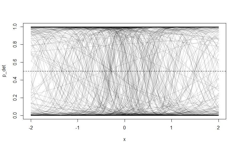
As we can see, something has gone badly wrong - nearly all of the prior probability is piled up on zero and one! The reason is that our priors are too flat. Remember that our priors are on the log-odds scale, and they will be turned into probability through the $logit$ link function. Because values below -4 and above 4 on the log-odds scale correspond to probabilities very close to 0 and 1 respectively, assigning a lot of our prior probability to these values by choosing a flat prior with a lot of area here makes the model assign a lot of prior probability to extreme values. Northrup and Gerber discuss this phenomenon in more detail in their paper, and offer recommendations for better priors. We’re going to try some tighter priors instead: $Normal(0,0.5)$ for $\alpha_{det}$ and $Normal(0,1)$ for $\beta_{W}$. If you modfy the code above to these values, then you get this plot:
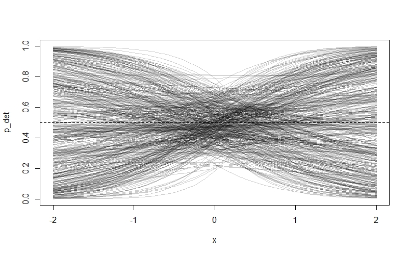
This looks much more sensible. We are also going to learn from this experience by choosing relatively tight priors for $\bar{k}$ and our $\beta$ values in the occupancy submodel: I’m going to suggest $Normal(0,0.2)$ and $Normal(0,1)$ respectively.
We’re going to use a similar strategy to choose priors for our Gaussian process parameters. However, in this case I find that it can be difficult to interpret lines drawn from the priors because of the way they plot over one-another, so I’m going to plot the compatability intervals instead:
samp <- 1e4
rho2_prior <- rexp(samp, 1)
eta2_prior <- rexp(samp, 1)

x_seq <- seq(0,4,0.01)
priorcov <- sapply(x_seq, function(x) eta2_prior * exp(-rho2_prior * x^2))
priorcov_mu <- apply(priorcov, 2, median)
priorcov_95CI <- apply(priorcov, 2, HPDI, prob=0.95)
priorcov_89CI <- apply(priorcov, 2, HPDI, prob=0.89)
priorcov_80CI <- apply(priorcov, 2, HPDI, prob=0.80)
priorcov_70CI <- apply(priorcov, 2, HPDI, prob=0.70)
priorcov_60CI <- apply(priorcov, 2, HPDI, prob=0.60)
priorcov_50CI <- apply(priorcov, 2, HPDI, prob=0.50)

par(mfrow=c(1,1))
plot(NULL, xlab="Distance", ylab="Covariance", xlim=c(0,4), ylim=c(0,2), main="Prior w/ Compatability Intervals")
lines(x_seq, priorcov_mu, lwd=2)
shade(priorcov_95CI, x_seq)
shade(priorcov_89CI, x_seq)
shade(priorcov_80CI, x_seq)
shade(priorcov_70CI, x_seq)
shade(priorcov_60CI, x_seq)
shade(priorcov_50CI, x_seq)
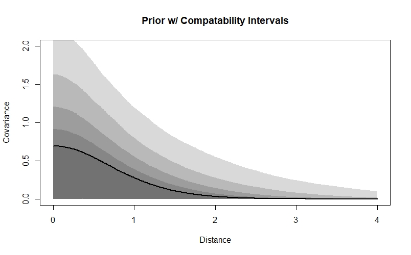
We can see that according to our priors, covariance will decline with distance, and will probably be low by the time that sites are 3 units apart - in a real dataset, we’d want to think about the distances between our sites and the scale that we’d expect autocorrelation to occur at when deciding whether these values are sensible. Our priors also assign more probability to smaller covariance values at each distance - they will be weakly regularising, meaning they are skeptical of more extreme values. However, they do allow for higher values if the data demand it.
Coding the model in Stan
Now that we’ve simulated from the data-generating process and chosen our priors, we’re ready to build our Stan model and fit it to the simulated data.
The full model
I’ll start by showing the Stan model in full. Don’t worry if it looks like a lot - we’re going to go through it step by step, and it’s really not as bad as it looks!
Here is the full model:
functions{
    matrix cov_GPL2(matrix x, real sq_alpha, real sq_rho, real delta) {
        int N = dims(x)[1];
        matrix[N, N] K;
        for (i in 1:(N-1)) {
          K[i, i] = sq_alpha + delta;
          for (j in (i + 1):N) {
            K[i, j] = sq_alpha * exp(-sq_rho * square(x[i,j]) );
            K[j, i] = K[i, j];
          }
        }
        K[N, N] = sq_alpha + delta;
        return K;
    }
}

data{
  int<lower=1> nsites; // Number of sites
  int<lower=1> N_maxvisits; // Maximum number of survey visits received by a site
  array[nsites] int<lower=1> V; // Number of visits per site

  array[nsites, N_maxvisits] int<upper=1> y; // Observed presence/absence data (NA's replaced with -9999)
  array[nsites] real x; // Occupancy covariate x
  array[nsites] real m; // Occupancy covariate m
  array[nsites, N_maxvisits] real w; // Detection covariate, varies with time (NA's replaced with -9999)

  matrix[nsites, nsites] dmat; // Distance matrix

}

parameters{
  // Effect sizes (on log-odds scale)
  real betax; // Occupancy slope (effect of x)
  real betam; // Occupancy slope (effect of m)
  real alphadet; // Detection intercept
  real betadet; // Detection slope (effect of w)
  real k_bar; // Average occupancy in entire population of sites

  // Gaussian process parameters
  vector[nsites] z; // z-scores for intercept term (for non-centred parameterisation)
  real<lower=0> etasq; // Maximum covariance between sites
  real<lower=0> rhosq; // Rate of decline in covariance with distance
}

transformed parameters{
  vector[nsites] psi; // Probability of occurrence at each site i
  array[nsites, N_maxvisits] real pij; // Probability of detection at each site i at each time j

  matrix[nsites, nsites] L_SIGMA; // Cholesky-decomposed covariance matrix
  matrix[nsites, nsites] SIGMA; // Covariance matrix
  vector[nsites] k; // Intercept term for each site (perturbation from k_bar)

 // Gaussian process - non-centred
  SIGMA = cov_GPL2(dmat, etasq, rhosq, 0.01);
  L_SIGMA = cholesky_decompose(SIGMA);
  k = L_SIGMA * z;

  // Calculate psi_i and pij
  for(isite in 1:nsites){
    // Occupancy submodel
    psi[isite] = inv_logit(k_bar + k[isite] + x[isite]*betax + m[isite]*betam);

    // Detection submodel
    for(ivisit in 1:V[isite]){
      pij[isite, ivisit] = inv_logit(alphadet + betadet*w[isite,ivisit]);
    }
  }

}

model{

  vector[nsites] log_psi; // Log of psi
  vector[nsites] log1m_psi; // Log of 1-psi

  // Priors
  betax ~ normal(0,1);
  betam ~ normal(0,1);
  alphadet ~ normal(0,0.5);
  betadet ~ normal(0,1);
  k_bar ~ normal(0,0.2);

  rhosq ~ exponential(1);
  etasq ~ exponential(1);
  z ~ normal(0, 1);

  // Log psi and log(1-psi)
  for(isite in 1:nsites){
    log_psi[isite] = log(psi[isite]);
    log1m_psi[isite] = log1m(psi[isite]);
  }

  // Likelihood
  for(isite in 1:nsites){

    if(sum(y[isite, 1:V[isite]]) > 0){
      target += log_psi[isite] + bernoulli_lpmf(y[isite, 1:V[isite]] | pij[isite, 1:V[isite]]);
    } else {
      target += log_sum_exp(log_psi[isite] + bernoulli_lpmf(y[isite, 1:V[isite]] | pij[isite, 1:V[isite]]), log1m_psi[isite]);
    }
  }// end likelihood contribution
}
Now let’s break it down, starting from the top.
The functions block
functions{
    matrix cov_GPL2(matrix x, real sq_alpha, real sq_rho, real delta) {
        int N = dims(x)[1];
        matrix[N, N] K;
        for (i in 1:(N-1)) {
          K[i, i] = sq_alpha + delta;
          for (j in (i + 1):N) {
            K[i, j] = sq_alpha * exp(-sq_rho * square(x[i,j]) );
            K[j, i] = K[i, j];
          }
        }
        K[N, N] = sq_alpha + delta;
        return K;
    }
}
This block, which I adapted from Statistical Rethinking, codes the kernel function $K_{i,j} = \eta^2exp(-\rho^2D^2_{i,j})$. You can customise the function by changing the line:
K[i, j] = sq_alpha * exp(-sq_rho * square(x[i,j]) );
The function also allows for a parameter called delta which I’ve chosen to ignore here. It represents the additional covariance that sites have with themselves (i.e., when $i=j$), and you can read more about it in Rethinking.
The data block
data{
  int<lower=1> nsites; // Number of sites
  int<lower=1> N_maxvisits; // Maximum number of survey visits received by a site
  array[nsites] int<lower=1> V; // Number of visits per site

  array[nsites, N_maxvisits] int<upper=1> y; // Observed presence/absence data (NA's replaced with -9999)
  array[nsites] real x; // Occupancy covariate x
  array[nsites] real m; // Occupancy covariate m
  array[nsites, N_maxvisits] real w; // Detection covariate, varies with time (NA's replaced with -9999)

  matrix[nsites, nsites] dmat; // Distance matrix
}
This block just tells Stan about the data which we supplied in dlist above. Have a look at str(dlist)and compare the output to the contents of the data block.
The parameters block
parameters{
  // Effect sizes (on log-odds scale)
  real betax; // Occupancy slope (effect of x)
  real betam; // Occupancy slope (effect of m)
  real alphadet; // Detection intercept
  real betadet; // Detection slope (effect of w)
  real k_bar; // Average occupancy in entire population of sites

  // Gaussian process parameters
  vector[nsites] z; // z-scores for intercept term (for non-centred parameterisation)
  real<lower=0> etasq; // Maximum covariance between sites
  real<lower=0> rhosq; // Rate of decline in covariance with distance
}
This block tells Stan about the model’s parameters, specifically the intercepts and effect sizes, and the parameters for the Gaussian process. Note that we have this weird z parameter which we’ve not seen before - this is for the non-centered parameterisation, which I’m going to cover in the next block.
The transformed parameters block
transformed parameters{
  vector[nsites] psi; // Probability of occurrence at each site i
  array[nsites, N_maxvisits] real pij; // Probability of detection at each site i at each time j

  matrix[nsites, nsites] L_SIGMA; // Cholesky-decomposed covariance matrix
  matrix[nsites, nsites] SIGMA; // Covariance matrix
  vector[nsites] k; // Intercept term for each site (perturbation from k_bar)

 // Gaussian process - non-centred
  SIGMA = cov_GPL2(dmat, etasq, rhosq, 0.01);
  L_SIGMA = cholesky_decompose(SIGMA);
  k = L_SIGMA * z;

  // Calculate psi_i and pij
  for(isite in 1:nsites){
    // Occupancy submodel
    psi[isite] = inv_logit(k_bar + k[isite] + x[isite]*betax + m[isite]*betam);

    // Detection submodel
    for(ivisit in 1:V[isite]){
      pij[isite, ivisit] = inv_logit(alphadet + betadet*w[isite,ivisit]);
    }
  }
}
Now we’re into some of the real action! We start off the transformed parameter blocks by defining a vector and array to hold the values for the occupancy probability $\psi_{i}$ for each site $i$ and the detection probability $p_{i,j}$ for each site $i$ at each survey $j$ respectively.
We then move onto a section which performs the Gaussian process part of the model, using the cov_GPL2 function we defined in the functions block. This section also uses a computational trick called non-centred parameterisation to make the model run better. I’m not going to go over the theory behind how this works here, but you can find out all about it in the Statistical Rethinking lectures here and here as well as in the book.
We first make some vectors and matrices to hold the Cholesky-decomposed covariance matrix L_SIGMA (for the non-centred parameterisation) as well as the regular old covariance matrix and intercepts for each site that we covered above. After this, we run the cov_GPL2 function, perform the Cholesky decomposition, and then multiply the resulting matrix L_SIGMAby the z scores we saw in the parameters block to obtain our intercept terms k.
In the final section, we calculate $\psi_{i}$ and $p_{i,j}$, looping over each site $i$ as well as each survey visit $j$ for the detection probability. This is the bit that contains the linear submodels for occupancy and detection. If you look at the two submodels, you can see the covariates we defined in the data block and the effect sizes from the parameters block. The occupancy submodel also contains the site-level intercept term $k_{i}$ as well as the average intercept term $\bar{k}$.
The model block
model{

  vector[nsites] log_psi; // Log of psi
  vector[nsites] log1m_psi; // Log of 1-psi

  // Priors
  betax ~ normal(0,1);
  betam ~ normal(0,1);
  alphadet ~ normal(0,0.5);
  betadet ~ normal(0,1);
  k_bar ~ normal(0,0.2);

  rhosq ~ exponential(1);
  etasq ~ exponential(1);
  z ~ normal(0, 1);

  // Log psi and log(1-psi)
  for(isite in 1:nsites){
    log_psi[isite] = log(psi[isite]);
    log1m_psi[isite] = log1m(psi[isite]);
  }

  // Likelihood
  for(isite in 1:nsites){

    if(sum(y[isite, 1:V[isite]]) > 0){
      target += log_psi[isite] + bernoulli_lpmf(y[isite, 1:V[isite]] | pij[isite, 1:V[isite]]);
    } else {
      target += log_sum_exp(log_psi[isite] + bernoulli_lpmf(y[isite, 1:V[isite]] | pij[isite, 1:V[isite]]), log1m_psi[isite]);
    }
  }// end likelihood contribution
}
Finally, we arrive at the model block. Again, there’s a lot going on in this section.
We first define two vectors to hold $log(\psi)$ and $1-log(\psi)$, which we’ll need in a minute.
We then move onto a section which defines the priors for each of our parameters. I picked the values for the priors based on the prior predictive simulations that we conducted above.
In the next section, we want to compute the likelihood, which will become part of the target (the log of the joint distribution of data and parameters) which is the thing that Stan actually samples. Unfortunately, there’s a problem - because Stan uses Hamiltonian Monte Carlo, we can’t use discrete parameters like the occupancy state $z_{i}$. We therefore need to get these parameters out of the model by marginalizing over them. Luckily, resources like this excellent tutorial by Maxwell B. Joseph explain how to do this! As my code here is adapted from the supplementary material of this paper by Allan Clark and Res Altwegg it appears very slightly different to Maxwell’s, but it does the same thing.
Running the model and exploring the output
Now that we’ve written the model, it’s time to run it! To do this, I use CmdStan via the cstan function in the rethinking package. First save the model as a .stan file (I called mine occ_gp_nc.stan) and then run the model like this:
m1_nc <- cstan(file = "C:/Stan_code/occupancy_models/occ_gp_nc.stan",
               data = dlist,
               chains = 4,
               cores = 4,
               warmup = 1500,
               iter = 2500,
               seed = 33221)
The model will now compile and sample. This could take a little while, so it’s a good idea to go for a walk / play with the dog / classify some of my camera trap photos ![]() until it’s done (relevant xkcd)!
until it’s done (relevant xkcd)!
When the sampling is complete, you’ll get a warning message saying that some variables have undefined values - this is safe to ignore, it’s just saying that there are no $p_{i,j}$ values for visits which were never conducted. We can now inspect some model diagnostics:
precis(m1_nc)
dashboard(m1_nc)
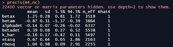
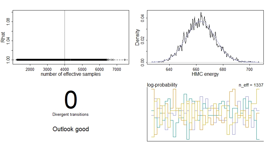
We’re particularly interested in the effective sample size n_effwhich should be some healthy number relative to our actual number of samples, the Gelman-Rubin convergence diagnostic Rhat which should be 1 for each parameter, and the number of divergent transitions which should ideally be zero. We should also inspect the traceplots for the key parameters here:
traceplot(m1_nc, pars=c("betax","betam","alphadet","betadet","k_bar","etasq","rhosq"))
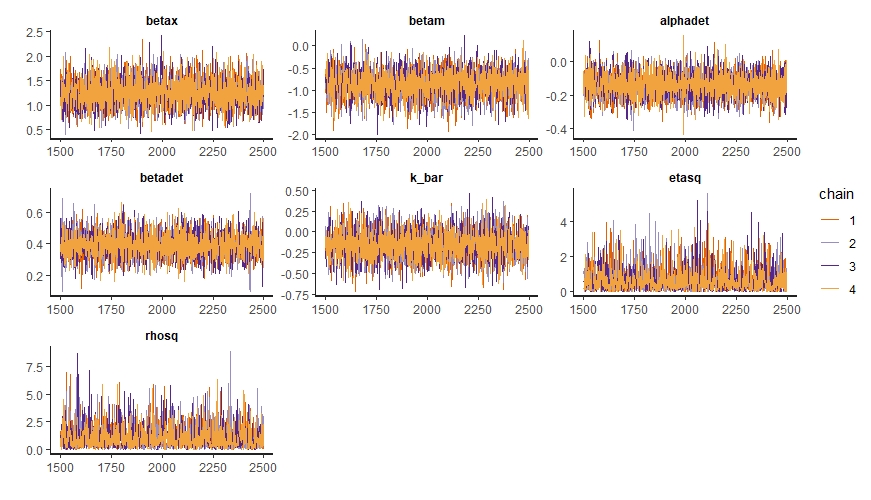
These ones look like “fuzzy caterpillars”, which is good.
Now that we’re happy that our model has performed adequately, we can extract our samples from the posterior distribution:
post <- extract.samples(m1_nc)
I think at this stage it’s a good idea to look inside our posterior distribution with str(post)to see what it looks like. We see that it’s a list, with a separate element for each of our parameters. We can see that there are 4000 samples for each parameter, because we ran 4 chains with 1000 iterations each (remember that we set iter=2500 but the 1500 warmup iterations don’t appear in post). If we look at some of the parameters, such as psi or SIGMA, we see that they have more dimensions - this is because they are vector or matrix parameters (e.g., psi is a vector with one value for each site). In total, we actually have 22400 parameters! Most of these (20000 of them) are for the covariance matrix SIGMA and the Cholesky-decomposed covariance matrix L_SIGMA.
Now that we’ve got our posterior distribution, we can start doing useful things with it! In the following sections, I go through a few of these things.
Looking at the key parameters
One of the first things we can do is look at the values for the key parameters in our model - the effect sizes ($\beta_{X},\beta{M},\beta{det}$), intercepts ($\alpha_{det},\bar{k}$), and the Gaussian process parameters ($\eta^2,\rho^2$). We can see these in the precis summary table but I prefer to look at them using density plots.
Since we simulated the data and know the true values of each parameter, we can also check to see whether the model estimated these values accurately. This is an important part of validating our model. An easy way to do this is to just add a vertical line to each density plot to show the true value:
par(mfrow=c(4,2))
dens(post$betax, main="betax"); abline(v=betax,lty=2)
dens(post$betam, main="betam"); abline(v=betam,lty=2)
dens(post$alphadet, main="alphadet"); abline(v=alphadet, lty=2)
dens(post$betadet, main="betadet"); abline(v=betadet, lty=2)
dens(post$k_bar, main="k_bar"); abline(v=0, lty=2)
dens(post$etasq, main="eta^2"); abline(v=eta2, lty=2)
dens(post$rhosq, main="rho^2"); abline(v=rho2, lty=2)
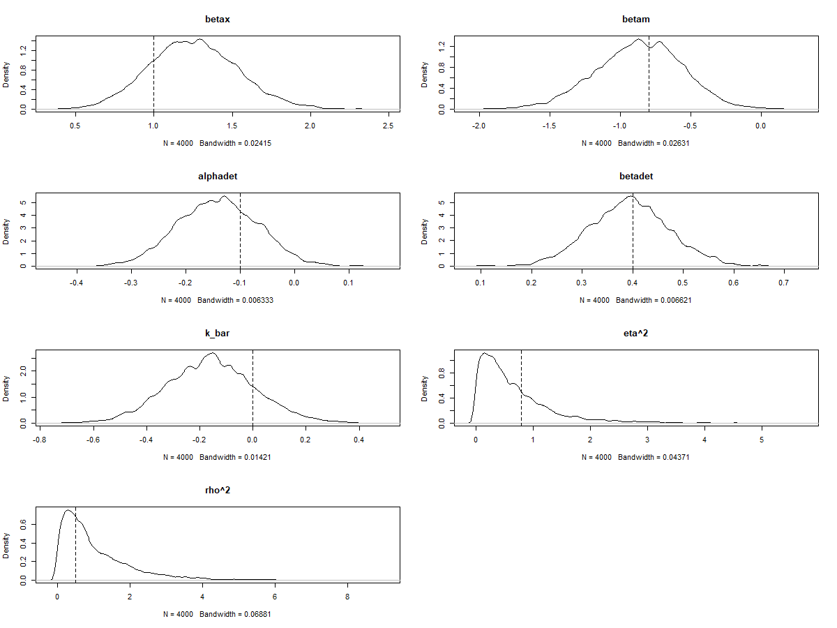
As you can see, in this example the model estimated all of the key parameters pretty accurately - the dashed vertical lines all fall somewhere within the posterior distribution for each parameter.
There’s a fair bit of uncertainty, but the model is still pretty good at identifying whether the effect size parameters are positive or negative - this is particularly important for betax, which is our effect of interest in this example.
Looking at the occupancy probability
We can also look at the model’s predictions of the occupancy probability at each site ($\psi_{i}$). Again, because we simulated the data we can compare this against the true value. Here I do this by plotting the posterior mean and 89% compatability intervals against the true value:
psi_mu <- apply(post$psi,2,mean)
psi_PI89 <- apply(post$psi, 2, HPDI, prob=0.89)

par(mfrow=c(1,1))
plot(NULL, xlim=c(0,1), ylim=c(0,1), xlab="True value", ylab="Model estimate", main=expression(psi))
abline(a=0,b=1, lty=2) # true = predicted
points(x = psi, y = psi_mu, pch=16, col=rangi2)
for(i in 1:length(psi)){
  lines(x = rep(psi[i],2), y = c(psi_PI89[1,i], psi_PI89[2,i]), col=rangi2)
}
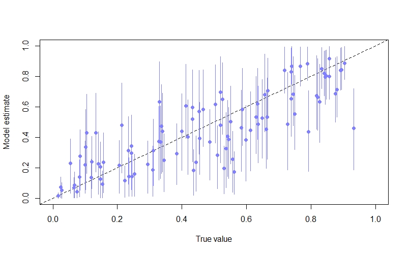
As we can see, the inferences are not too bad, with many of the points lying close to the diagonal line where the model’s estimate is equal to the true value.
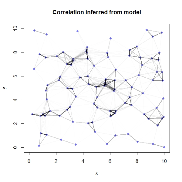
Visualising the spatial autocorrelation
One of the really cool things we can do is visualise the spatial autocorrelation between sites. The first thing we need to do here is to compute the posterior median covariance among sites (i.e., the most probable covariance matrix according to the model) and convert it into a correlation matrix:
K <- matrix(0, nrow=sites, ncol=sites)
for(i in 1:sites){
  for(j in 1:sites){
    K[i,j] <- median(post$etasq) * exp(-median(post$rhosq)*dmat2[i,j])
  }
}
diag(K) <- median(post$etasq) + 0.01

Rho <- round(cov2cor(K),2)
rownames(Rho) <- seq(1,100,1)
colnames(Rho) <- rownames(Rho)
We can now plot the results on a map, with darker lines representing a higher degree of correlation between sites:
par(mfrow=c(1,1))
plot(y~x, data=coords, col=rangi2, pch=16, xlim=c(0,10), ylim=c(0,10), main="Correlation inferred from model")

for(i in 1:sites){
  for(j in 1:sites){
    if(i < j){
      lines(x = c(coords$x[i], coords$x[j]),
            y = c(coords$y[i], coords$y[j]),
            lwd=2, col=col.alpha("black", Rho[i,j]^2))
    }
  }
}
Again, because we simulated the data we are able to compare our model’s results against the truth:
# Compute true correlation matrix
Rho_t <- round(cov2cor(covmat),2)
rownames(Rho_t) <- seq(1,100,1)
colnames(Rho_t) <- rownames(Rho)

# Plot correlations on a map
plot(y~x, data=coords, col=rangi2, pch=16, xlim=c(0,10), ylim=c(0,10), main="True correlation")

for(i in 1:sites){
  for(j in 1:sites){
    if(i < j){
      lines(x = c(coords$x[i], coords$x[j]),
            y = c(coords$y[i], coords$y[j]),
            lwd=2, col=col.alpha("black", Rho_t[i,j]^2))
    }
  }
}
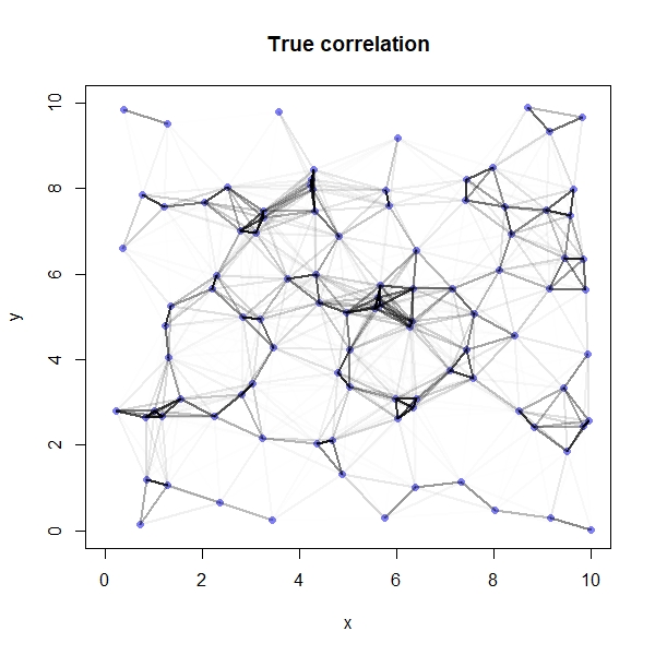
We see that our model has done a great job here - the two plots looks pretty similar!
Simulating an intervention
The effect of intervening in the system (i.e., changing the value of $X$) on the occupancy probability is often different to the effect size for the covariate of interest (i.e., $\beta_{X}$). This is because when there are extreme values for other covariates the occupancy probabilty can get pushed close to zero or one, making the effect of our focal covariate less important - this is a floor/ceiling effect.
The consequence is that if we’re interested in understanding the consequences of changing $X$, then we have to consider how the other variables which effect occupancy (in this case, $M$) are distributed. One way of dealing with this challenge is by using a simulation.
The exact code for our simulation depends on whether we’re interested in simulating an intervention for the specific sites that we surveyed, or for the (hypothetical) population of all sites. We’ll start with the specific sites we surveyed:
# Simulating intervention for the sites that we surveyed
simsites <- sites # There were 100 sites that we surveyed
nsamples <- 4000 # Number of samples from posterior to use (4000 = all of them)

# Matrices to store our results
S1 <- matrix(0, nrow=nsamples, ncol=simsites)
S2 <- matrix(0, nrow=nsamples, ncol=simsites)

new_x <- x + 1 # Simulate increasing x by 1

# Under status quo
for(s in 1:simsites){
  inv_psi <- post$k_bar + post$k[,s] + post$betax*x[s] + post$betam*m[s]
  psi_sim <- inv_logit(inv_psi)
  S1[,s] <- psi_sim
}

# Under distribution of x after intervention
for(s in 1:simsites){
  inv_psi <- post$k_bar + post$k[,s] + post$betax*new_x[s] + post$betam*m[s]
  psi_sim <- inv_logit(inv_psi)
  S2[,s] <- psi_sim
}

# Difference between distribution under the two scenarios
Sdiff <- S2-S1
dens(Sdiff)
abline(v=inv_logit(betax)-inv_logit(0), lty=2) # true betax
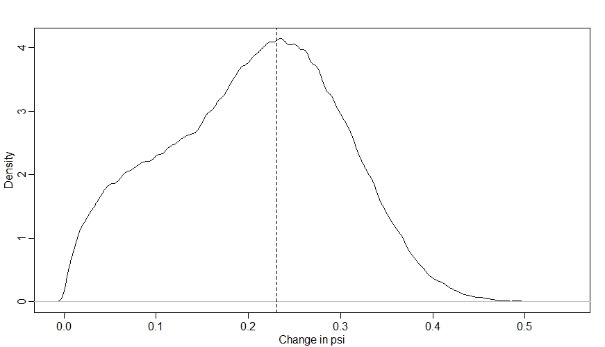
Looking at this distribution, we can see that there is a fair amount of uncertainty in what will happen to $\psi$ when we increase $X$ by 1, but the model is pretty sure that the effect of the intervention will be to increase $\psi$. The peak of our distribution is at around 0.23, which is what we’d expect from our $\beta_{X}$ parameter (as when $\bar{k}$ is 0, the true effect of $X$ is an increase $\psi$ from 0 to 1 on the log-odds scale, which is an increase from 0.5 to 0.73 on the probabilty scale, i.e. an increase of 0.23 - I’ve shown this value with a dashed vertical line).
However, notice that the distribution is not symmetrical - for some of the sites, increasing $X$ had less of an effect on $\psi$. This is due to ceiling and floor effects that occur at some sites where both the values of $k$ and $M$ are relatively extreme.
Now let’s look at simulating the intervention for the hypothetical population of all sites. The approach is generally similar to what we’ve just done, but there are a couple of key differences. The first is that we no longer need to use our $k_{i}$ values. The second is that we need to decide on a distribution for $M$ to average over - here I’ve gone for $Uniform(0,4)$ because it’ll really exaggerate the ceiling/floor effects, which will be interesting to see:
# Simulating intervention for hypothetical population of sites
simsites <- 5000 # 5000 hypothetical sites
nsamples <- 4000 # Number of samples from posterior to use (4000 = all of them)

# Matrices to store our results
S1 <- matrix(0, nrow=nsamples, ncol=simsites)
S2 <- matrix(0, nrow=nsamples, ncol=simsites)

old_x <- rnorm(simsites, 0, 1)
new_x <- old_x + 1 # Simulate increasing x by 1
m_sim <- runif(simsites, 0, 4)

# Under status quo
for(s in 1:simsites){
  inv_psi <- post$k_bar + post$betax*old_x[s] + post$betam*m_sim[s]
  psi_sim <- inv_logit(inv_psi)
  S1[,s] <- psi_sim
}

# Under distribution of x after intervention
for(s in 1:simsites){
  inv_psi <- post$k_bar + post$betax*new_x[s] + post$betam*m_sim[s]
  psi_sim <- inv_logit(inv_psi)
  S2[,s] <- psi_sim
}

Sdiff <- S2-S1

dens(Sdiff)
abline(v=inv_logit(betax)-inv_logit(0), lty=2)
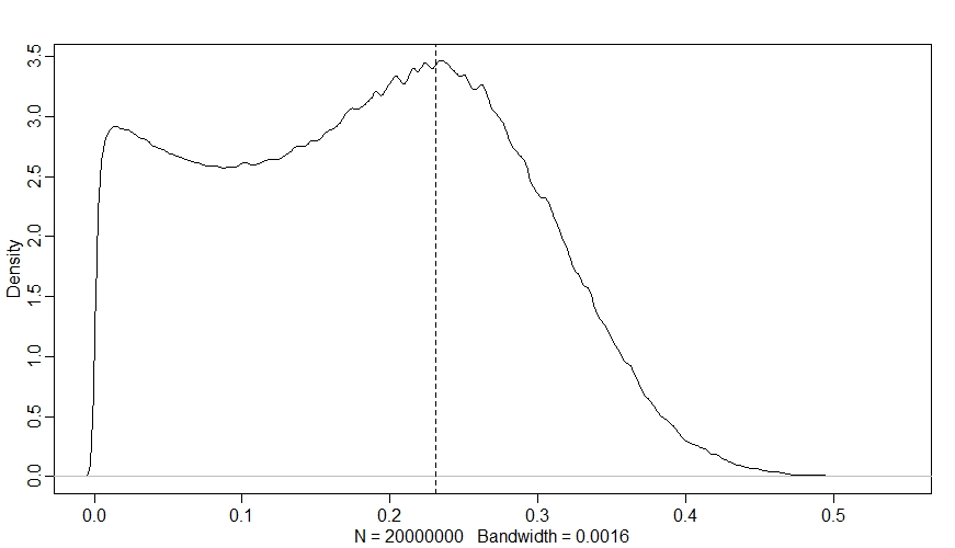
Now we can really see the ceiling and floor effects - in a large proportion of sites, changing $X$ had almost no effect on $\psi$, even though $\beta_{X}$ is strongly positive! Since $k_{i}$ is out of the picture now, this is all down to $M$ - we can see this if we plot the change in $\psi$ against $M$ like so:
plot(NULL, xlim=range(m_sim), ylim=c(-0.5,0.5), ylab="Change in psi",xlab="m_sim")
abline(h=0, lty=2)
for(s in 1:simsites){
  points(m_sim[s], mean(Sdiff[,s]))
}
ate <- mean(Sdiff) # Average treatment effect
abline(h=ate,lwd=2)
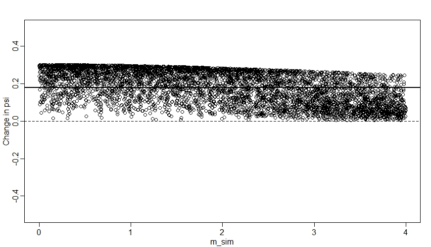
We can see here that when $M$ (m_sim) is high, the change in $\psi$ tends to be closer to zero.
Comments